Tutorial¶

The hierarchical ensemble methods proposed in HEMDAG package can be run by using any ontology listed in OBO foundry (link). In this tutorial we perform experiments by using the Human Phenotype Ontology (HPO, link) and the Gene Ontology (GO, link).

Note

The experiments run on this tutorial were executed by using the HEMDAG version 2.6.0, the R version 3.6.1 and on a machine having Ubuntu 16.04 as operative system.

Hierarchical Prediction of HPO terms¶

Here we show a step-by-step application of HEMDAG to the hierarchical prediction of associations between human gene and abnormal phenotype. To this end we will use the small pre-built dataset available in the HEMDAG library. Nevertheless, you can perform the examples shown below by using the full dataset available at the following link.

Note

By using the full dataset the running time of the parametric ensemble variants is quite higher due to the tuning of the hyper-parameters…

Reminder. To load the HEMDAG library in the R environment, just type:

library(HEMDAG);

and to load an rda file in the R environment just type:

load("file_name.rda");

Loading the Flat Scores Matrix¶

In their more general form, the hierarchical ensemble methods adopt a two-step learning strategy: the first step consists in the flat learning of the ontology terms, while the second step reconciles the flat predictions by considering the topology of the ontology. Hence, the first ingredient that we need is the flat scores matrix. For the sake of simplicity, in the examples shown below we make use of the pre-built dataset available in the HEMDAG library. To load the flat scores matrix, open the R environment and type:

data(scores);

with the above command we loaded the flat scores matrix S, that is a named 100 X 23 matrix. Rows correspond to genes (Entrez GeneID) and columns to HPO terms/classes. The scores representing the likelihood that a given gene belongs to a given class: the higher the value, the higher the likelihood that a gene belongs to a given class. This flat scores matrix was obtained by running the RANKS package (link).

Loading the DAG¶

In order to know the hierarchical structure of the HPO terms, we must load the graph:

data(graph);

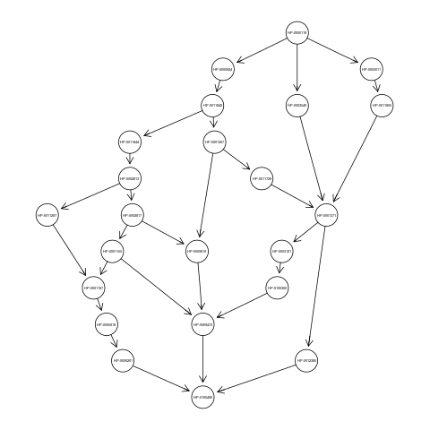
with the above command we loaded the graph g, an object of class graphNEL. The graph g has 23 nodes and 30 edges and represents the ancestors view of the HPO term Camptodactyly of finger (HP:0100490). Nodes of the graph g must correspond to classes of the flat scores matrix S.

Optional step: plotting the graph `g`¶

Note

To plot the graph you need to install before the Rgraphviz package. Yo can install this library for example by conda (conda install -c bioconda bioconductor-rgraphviz) or by Bioconductor (link).

If you want to visualize the ancestors view of the term HP:0100490, just type:

library(Rgraphviz);
plot(g);

Scores Normalization¶

If the flat classifier used as base learner in HEMDAG library returns a score and not a probability, we must normalize the scores of the flat matrix to make the flat scores comparable with the hierarchical ones. HEMDAG allows to normalize the flat scores according to two different procedures:

MaxNorm: Normalization in the sense of the maximum: the score of each class is normalized by dividing the score values for the maximum score of that class:

maxnorm <- normalize.max(S);

Qnorm: Quantile normalization: quantile normalization of the preprocessCore package is used:

library(preprocessCore);
qnrom <- normalize.quantiles(S);

Be sure to install the preprocessCore package before running the above command. Yo can install it by conda (conda install -c bioconda bioconductor-preprocesscore) or by Bioconductor (link)

For the examples shown below, we normalize the flat scores matrix by applying the MaxNorm:

S <- normalize.max(S);

Running Hierarchical Ensemble Methods¶

First of all, we need to find the root node (i.e. node that is at the top-level of the hierarchy) of the HPO graph g. To do that just type:

root <- root.node(g);

in this way we store in the variable root the root node of the graph g.

Now, we are ready to run any ensemble algorithms implemented in the HEMDAG package. Depending on which ensemble variant you want to call, you must execute one of the command listed below:

HTD-DAG: Hierarchical Top Down for DAG¶

S.htd <- htd(S,g,root);

GPAV-DAG: Generalized Pool-Adjacent-Violators for DAG¶

S.gpav <- GPAV.over.examples(S, W=NULL, g);

TPR-DAG: True Path Rule for DAG¶

TPR-DAG is a family of algorithms according to the bottom-up approach adopted for the choice of the positive children. In the top-down step (that guarantees coherent predictions with the ontology ones) TPR-DAG strategy uses the HTD-DAG algorithm.

S.tprTF    <- TPR.DAG(S, g, root, positive="children", bottomup="threshold.free", topdown="HTD");
S.tprT     <- TPR.DAG(S, g, root, positive="children", bottomup="threshold", topdown="HTD", t=0.5);
S.tprW     <- TPR.DAG(S, g, root, positive="children", bottomup="weighted.threshold.free", topdown="HTD", w=0.5);
S.tprWT    <- TPR.DAG(S, g, root, positive="children", bottomup="weighted.threshold", topdown="HTD", t=0.5, w=0.5);

ISO-TPR: Isotonic Regression for DAG¶

TPR-DAG is a family of algorithms according to the bottom-up approach adopted for the choice of the positive children. To make scores consistent with the ontology predictions ISO-TPR employs in the top-down step the GPAV-DAG algorithm.

S.ISOtprTF <- TPR.DAG(S, g, root, positive="children", bottomup="threshold.free", topdown="GPAV");
S.ISOtprT  <- TPR.DAG(S, g, root, positive="children", bottomup="threshold", topdown="GPAV", t=0.5);
S.ISOtprW  <- TPR.DAG(S, g, root, positive="children", bottomup="weighted.threshold.free", topdown="GPAV", w=0.5);
S.ISOtprWT <- TPR.DAG(S, g, root, positive="children", bottomup="weighted.threshold", topdown="GPAV", t=0.5, w=0.5);

DESCENS: Descendants Ensemble Classifier¶

DESCENS is a family of algorithms according to the bottom-up approach adopted for the choice of the positive descendants. In the top-down step DESCENS uses the HTD-DAG algorithm.

S.descensTF     <- TPR.DAG(S, g, root, positive="descendants", bottomup="threshold.free", topdown="HTD");
S.descensT      <- TPR.DAG(S, g, root, positive="descendants", bottomup="threshold", topdown="HTD", t=0.5);
S.descensW      <- TPR.DAG(S, g, root, positive="descendants", bottomup="weighted.threshold.free", topdown="HTD", w=0.5);
S.descensWT     <- TPR.DAG(S, g, root, positive="descendants", bottomup="weighted.threshold", topdown="HTD", t=0.5, w=05);
S.descensTAU    <- TPR.DAG(S, g, root, positive="descendants", bottomup="tau", topdown="HTD", t=0.5);
S.ISOdescensTF  <- TPR.DAG(S, g, root, positive="descendants", bottomup="threshold.free", topdown="GPAV");
S.ISOdescensT   <- TPR.DAG(S, g, root, positive="descendants", bottomup="threshold", topdown="GPAV", t=0.5);
S.ISOdescensW   <- TPR.DAG(S, g, root, positive="descendants", bottomup="weighted.threshold.free", topdown="GPAV", w=0.5);
S.ISOdescensWT  <- TPR.DAG(S, g, root, positive="descendants", bottomup="weighted.threshold", topdown="HTD", t=0.5, w=05);
S.ISOdescensTAU <- TPR.DAG(S, g, root, positive="descendants", bottomup="tau", topdown="GPAV", t=0.5);

ISO-DESCENS: Isotonic Regression with Descendants Ensemble Classifier¶

ISO-DESCENS is a family of algorithms according to the bottom-up approach adopted for the choice of the positive descendants. For the top-down step ISO-DESCENS employs the GPAV-DAG algorithm.

S.ISOdescensTF  <- TPR.DAG(S, g, root, positive="descendants", bottomup="threshold.free", topdown="GPAV");
S.ISOdescensT   <- TPR.DAG(S, g, root, positive="descendants", bottomup="threshold", topdown="GPAV", t=0.5);
S.ISOdescensW   <- TPR.DAG(S, g, root, positive="descendants", bottomup="weighted.threshold.free", topdown="GPAV", w=0.5);
S.ISOdescensWT  <- TPR.DAG(S, g, root, positive="descendants", bottomup="weighted.threshold", topdown="HTD", t=0.5, w=05);
S.ISOdescensTAU <- TPR.DAG(S, g, root, positive="descendants", bottomup="tau", topdown="GPAV", t=0.5);

Obozinski Heuristic Methods¶

S.max <- heuristic.max(S,g,root);
S.and <- heuristic.and(S,g,root);
S.or  <- heuristic.or(S,g,root);

Hierarchical Constraints Check¶

The predictions returned by our ensemble methods always obey to the True Path Rule: positive instance for a class implies positive instance for all the ancestors of that class. To check this fact we can apply the function check.hierarchy:

check.hierarchy(S,g,root)$Status
[1] "NOTOK"

check.hierarchy(S.htd,g,root)$Status
[1] "OK"

Obviously, all the ensemble variants hold this property, for instance:

check.hierarchy(S.tprTF,g,root)$Status
[1] "OK"

check.hierarchy(S.descensW,g,root)$Status
[1] "OK"

Performance Evaluation¶

To know the ensemble methods behavior, the HEMDAG library, by using precrec package, provides several performance metrics:

AUROC: area under the ROC curve;
AUPRC: area under the precision-recall curve;
F-max: maximum hierarchical F-score [Jiang2016];
PXR : precision at different recall levels;

Note

HEMDAG allows to compute all the aforementioned performance metrics either one-shot or averaged across k fold. Depending on the size of your dataset, the metrics F-max and PXR could take a while to finish. Please refer to HEMDAG reference manual for further information about what these functions receive in input and return in output.

[Jiang2016]

Jiang et al., An expanded evaluation of protein function prediction methods shows an improvement in accuracy, Genome Biology, vol. 17, p. 184, 2016

Loading the Annotation Matrix¶

To compare the hierarchical ensemble methods against the flat approach, we need of the annotation matrix:

data(labels);

with the above command we loaded the annotations table L, that is a named 100 X 23 matrix. Rows correspond to genes (Entrez GeneID) and columns to HPO terms/classes. L[i, j] = 1 means that the gene i belong to class j, L[i, j] = 0 means that the gene i does not belong to class j.

Flat vs Hierarchical¶

Before computing performance metrics we must remove the root node from the annotation matrix, the flat scores matrix and the hierarchical scores matrix. It does not make sense at all to take into account the predictions of the root node, since it is a dummy node added to the ontology for practical reasons (e.g. some graph-based software may require a single root node to work). In R this can be accomplished in one line of code.

## remove root node from annotation matrix
if(root %in% colnames(L))
    L <- L[,-which(colnames(L)==root)];

## remove root node from flat scores matrix
if(root %in% colnames(S))
    S <- S[,-which(colnames(S)==root)];

## remove root node from hierarchical scores matrix (eg S.htd)
if(root %in% colnames(S.htd))
    S.htd <- S.htd[,-which(colnames(S.htd)==root)];

Now we can compare the flat approach RANKS versus e.g. HTD-DAG by averaging the performance across 3 folds:

## FLAT
PRC.flat <- AUPRC.single.over.classes(L, S, folds=3, seed=1);
AUC.flat <- AUROC.single.over.classes(L, S, folds=3, seed=1);
PXR.flat <- precision.at.given.recall.levels.over.classes(L, S, recall.levels=seq(from=0.1, to=1, by=0.1), folds=3, seed=1);
FMM.flat <- compute.Fmeasure.multilabel(L, S, n.round=3, f.criterion="F", verbose=FALSE, b.per.example=TRUE, folds=3, seed=1);

## HIERARCHICAL
PRC.hier <- AUPRC.single.over.classes(L, S.htd, folds=3, seed=1);
AUC.hier <- AUROC.single.over.classes(L, S.htd, folds=3, seed=1);
PXR.hier <- precision.at.given.recall.levels.over.classes(L, S.htd, recall.levels=seq(from=0.1, to=1, by=0.1), folds=3, seed=1);
FMM.hier <- compute.Fmeasure.multilabel(L, S.htd, n.round=3, f.criterion="F", verbose=FALSE, b.per.example=TRUE, folds=3, seed=1);

By looking at the results we can see that HTD-DAG outperforms the flat classifier RANKS:

## AUC performance: flat vs hierarchical
 AUC.flat$average
 [1] 0.8263
 AUC.hier$average
 [1] 0.8312

 ## PRC performance: flat vs hierarchical
 PRC.flat$average
 [1] 0.4373
 PRC.hier$average
 [1] 0.4827

 ## F-score performance: flat vs hierarchical
 FMM.flat$average
    P      R      S      F      avF    A      T
 0.7071 0.6443 0.6853 0.6743 0.5768 0.7314 0.7020
 FMM.hier$average
    P      R      S      F      avF    A      T
 0.5087 0.9394 0.4430 0.6600 0.5922 0.6570 0.4457

 ## Precision at different recall levels: flat vs hierarchical
 PXR.flat$avgPXR
    0.1    0.2    0.3    0.4    0.5    0.6    0.7    0.8    0.9    1
 0.5872 0.5872 0.5872 0.5715 0.5715 0.4487 0.4361 0.4361 0.4361 0.4361
 PXR.hier$avgPXR
    0.1    0.2    0.3    0.4    0.5    0.6    0.7    0.8    0.9    1
 0.6465 0.6465 0.6465 0.6227 0.6227 0.4996 0.4897 0.4897 0.4897 0.4897

Note

HTD-DAG is the simplest ensemble approach among those available. HTD-DAG strategy makes flat scores consistent with the hierarchy by propagating from to top to the bottom of the hierarchy the negative predictions. Hence, in the worst case might happen that the predictions at leaves nodes are all negatives. Other ensemble variants (such as GPAV-DAG and TPR-DAG and its variants) lead to better improvements.

Running Experiments with the Hierarchical Ensemble Methods¶

The HEMDAG library provides also high-level functions for batch experiments, where input and output data must be stored in compressed rda files. In this way we can run experiment with different ensemble variants by properly changing the arguments of high-level functions implemented in HEMDAG:

Do.HTD: high-level function to run experiments with HTD-DAG algorithm;
Do.GPAV: high-level function to run experiments with GPAV-DAG algorithm;
Do.TPR.DAG: high-level function to run experiments with all TPR-DAG variants;
Do.HTD.holdout: high-level function to run hold-out experiment with HTD-DAG algorithm;
Do.GPAV.holdout: high-level function to run hold-out experiment with GPAV-DAG algorithm;
Do.TPR.DAG.holdout: high-level function to run hold-out experiment with all TPR-DAG variants;

The normalization can be applied on-the-fly within the ensemble high-level function or can be pre-computed through the function Do.flat.scores.normalization. Please have a look to the reference manual for further details on this function.

Cross-Validated Experiments¶

Here we perform several experiments by using the high-level functions, which provide an user-friendly interface to facilitate the execution of hierarchical ensemble methods.

Data Preparation¶

For the following experiments we store the input data (i.e. the flat scores matrix S, the graph g and the annotation table L) in the directory data and the output data (i.e. the hierarchical scores matrix and the performances) in the folder results:

# load data
data(graph);
data(scores);
data(labels);

if(!dir.exists("data"))
    dir.create("data");

if(!dir.exists("results"))
    dir.create("results");

# store data
save(g,file="data/graph.rda");
save(L,file="data/labels.rda");
save(S,file="data/scores.rda");

HTD-DAG Experiments¶

Here we perform exactly the same experiment that we did above, but using this time the high-level Do.HTD to compute the HTD-DAG algorithm:

Do.HTD( norm=FALSE, norm.type="MaxNorm", folds=3, seed=1, n.round=3, f.criterion="F",
        recall.levels=seq(from=0.1, to=1, by=0.1), flat.file="scores", ann.file="labels",
        dag.file="graph", flat.dir="data/", ann.dir="data/", dag.dir="data/",
        hierScore.dir="results/", perf.dir="results/", compute.performance=TRUE);

Obviously the results returned by Do.HTD are identical to those obtained by the step-by-step experiment performed above:

load("results/PerfMeas.MaxNorm.scores.hierScores.HTD.rda");

## AUC performance: flat vs hierarchical
AUC.flat$average
[1] 0.8263
AUC.hier$average
[1] 0.8312

## PRC performance: flat vs hierarchical
PRC.flat$average
[1] 0.4373
PRC.hier$average
[1] 0.4827

## F-score performance: flat vs hierarchical
FMM.flat$average
   P      R      S      F      avF    A      T
0.7071 0.6443 0.6853 0.6743 0.5768 0.7314 0.7020
FMM.hier$average
   P      R      S      F      avF    A      T
0.5087 0.9394 0.4430 0.6600 0.5922 0.6570 0.4457

## Precision at different recall levels: flat vs hierarchical
PXR.flat$avgPXR
   0.1    0.2    0.3    0.4    0.5    0.6    0.7    0.8    0.9    1
0.5872 0.5872 0.5872 0.5715 0.5715 0.4487 0.4361 0.4361 0.4361 0.4361
PXR.hier$avgPXR
   0.1    0.2    0.3    0.4    0.5    0.6    0.7    0.8    0.9    1
0.6465 0.6465 0.6465 0.6227 0.6227 0.4996 0.4897 0.4897 0.4897 0.4897

Note

All the high-level functions running ensemble-based algorithms automatically remove the root node from the annotation matrix, the flat and the hierarchical scores matrix before computing performance metrics.

GPAV-DAG Experiments¶

Burdakov et al. in [Burdakov06] proposed an approximate algorithm, named GPAV, to solve the isotonic regression (IR) or monotonic regression (MR) problem in its general case (i.e. partial order of the constraints). GPAV algorithm combines both low computational complexity (estimated to be \(\mathcal{O}(|V|^2)\)) and high accuracy.

[Burdakov06]

Sysoev, A. Grimvall, and O. Burdakov, Data preordering in generalized pav algorithm for monotonic regression, Journal of Computational Mathematics, vol. 24, no. 6, pp. 771–790, 2006

To run experiments with GPAV-DAG we must type, for instance:

Do.GPAV( norm=FALSE, norm.type= "MaxNorm", W=NULL, parallel=TRUE, ncores=7,
         folds=3, seed=1, n.round=3, f.criterion ="F", flat.file="scores",
         recall.levels=seq(from=0.1, to=1, by=0.1), ann.file="labels",
         dag.file="graph", flat.dir="data/", ann.dir="data/", dag.dir="data/",
         hierScore.dir="results/", perf.dir="results/", compute.performance=TRUE);

By loading the GPAV-DAG performance results we can see that this ensemble variant outperforms the flat classifier RANKS:

load("results/PerfMeas.MaxNorm.scores.hierScores.GPAV.rda");

## AUC performance: flat vs hierarchical
AUC.flat$average
[1] 0.8263
AUC.hier$average
[1] 0.8438

## PRC performance: flat vs hierarchical
PRC.flat$average
[1] 0.4373
PRC.hier$average
[1] 0.5201

## F-score performance: flat vs hierarchical
FMM.flat$average
     P      R      S      F    avF      A      T
0.7071 0.6443 0.6853 0.6743 0.5768 0.7314 0.7020
FMM.hier$average
     P      R      S      F    avF      A      T
0.5893 0.8581 0.5311 0.6988 0.6009 0.6983 0.5360

## Precision at different recall levels: flat vs hierarchical
PXR.flat$avgPXR
   0.1    0.2    0.3    0.4    0.5    0.6    0.7    0.8    0.9      1
0.5872 0.5872 0.5872 0.5715 0.5715 0.4487 0.4361 0.4361 0.4361 0.4361
PXR.hier$avgPXR
   0.1    0.2    0.3    0.4    0.5    0.6    0.7    0.8    0.9      1
0.6976 0.6976 0.6976 0.6835 0.6835 0.5214 0.5005 0.5005 0.5005 0.5005

TPR-DAG and ISO-TPR experiments¶

TPR-DAG is a family of algorithms in according to the chosen bottom-up and top-down approach. There are both parametric and non-parametric variants. To change variant is sufficient to modify the argument of the following parameters of the Do.TPR.DAG high-level function:

threshold;
weight;
positive;
topdown;
bottomup;

Please refer to the reference manual for further details about these parameters.

By replacing GPAV-DAG with HTD-DAG in the top-down step of TPR-DAG (variable topdown), we design the ISO-TPR algorithm. The most important feature of ISO-TPR is that it maintains the hierarchical constraints by construction and selects the closest solution (in the least square sense) to the bottom-up predictions that obey the true path rule, the logical and biological rule that govern the bio-ontology, such as HPO and GO.

Below we perform several experiments by playing with different TPR-DAG and ISO-TPR ensemble variants. In all the experiments, the performances were averaged across 3 folds.

Note

In Do.TPR-DAG high-level function the parameter kk refers to the number of folds of the cross validation on which tuning the parameters of the parametric variants of the hierarchical ensemble algorithms, whereas the parameter folds refers to number of folds of the cross validation on which computing the performance metrics averaged across folds. For the non-parametric variants (i.e. if bottomup = threshold.free), Do.TPR-DAG automatically set to zero the parameters kk and folds.

ISOtprT: flat scores matrix normalized by MaxNorm, positive children selection (normalizing the threshold on AUPRC (PRC) across 5 folds, parameter kk=5) and by applying GPAV-DAG strategy in the top-down step

Do.TPR.DAG( threshold=seq(0.1,0.9,0.1), weight=0, kk=5, folds=3, seed=1, norm=FALSE,
            norm.type="MaxNorm", positive="children", bottomup="threshold", topdown="GPAV",
            n.round=3, f.criterion="F", metric="PRC", recall.levels=seq(from=0.1, to=1, by=0.1),
            flat.file="scores", ann.file="labels", dag.file="graph", flat.dir="data/",
            ann.dir="data/", dag.dir="data/", hierScore.dir="results/",
            perf.dir="results/", compute.performance=TRUE);

ISOdescensTF: flat scores matrix normalized by MaxNorm, positive descendants selection (without threshold) and by applying GPAV-DAG strategy in the top-down step

Do.TPR.DAG( threshold=0, weight=0, kk=NULL, folds=3, seed=73, norm=FALSE, norm.type="MaxNorm",
            positive="descendants", bottomup="threshold.free", topdown="GPAV", n.round=3,
            f.criterion="F", metric=NULL, recall.levels=seq(from=0.1, to=1, by=0.1),
            flat.file="scores", ann.file="labels", dag.file="graph", flat.dir="data/",
            ann.dir="data/", dag.dir="data/", hierScore.dir="results/",
            perf.dir="results/", compute.performance=TRUE);

ISOdescensTAU: flat scores matrix normalized by Qnorm, positive descendants selection (maximizing the threshold on the F-score (FMAX) across 5 folds, parameter kk=5)and by applying GPAV-DAG strategy in the top-down step

Do.TPR.DAG( threshold=seq(0.1,0.9,0.1), weight=0, kk=5, folds=3, seed=1, norm=FALSE,
            norm.type="Qnorm", positive="descendants", bottomup="tau", topdown="GPAV",
            n.round=3, f.criterion="F", metric="FMAX", flat.file="scores",
            ann.file="labels", recall.levels=seq(from=0.1, to=1, by=0.1),
            dag.file="graph", flat.dir="data/", ann.dir="data/", dag.dir="data/",
            hierScore.dir="results/", perf.dir="results/", compute.performance=TRUE);

tprT: flat scores matrix normalized by Qnorm, positive children selection (maximizing the threshold on the F-score (FMAX) across 5 folds, parameter kk=5) and by applying HTD-DAG strategy in the top-down step

Do.TPR.DAG( threshold=seq(0.1,0.9,0.1), weight=0, kk=5, folds=3, seed=1, norm=FALSE,
            norm.type="Qnorm", positive="children", bottomup="threshold", topdown="HTD",
            n.round=3, f.criterion="F", metric="FMAX", recall.levels=seq(from=0.1, to=1, by=0.1),
            flat.file="scores", ann.file="labels", dag.file="graph", flat.dir="data/",
            ann.dir="data/", dag.dir="data/", hierScore.dir="results/",
            perf.dir="results/", compute.performance=TRUE);

descensW: flat scores matrix normalized by MaxNorm,*positive* descendants selection (maximizing the weight on the F-score (FMAX) across 5 folds, parameter kk=5) and by applying HTD-DAG strategy in the top-down step

Do.TPR.DAG( threshold=0, weight=seq(0.1,0.9,0.1), kk=5, folds=3, seed=1, norm=FALSE,
            norm.type="MaxNorm", positive="descendants", bottomup="weighted.threshold.free",
            topdown="GPAV", n.round=3, f.criterion="F", metric="FMAX", flat.file="scores",
            recall.levels=seq(from=0.1, to=1, by=0.1), ann.file="labels", dag.file="graph",
            flat.dir="data/", ann.dir="data/", dag.dir="data/", hierScore.dir="results/",
            perf.dir="results/", compute.performance=TRUE);

descensTF: flat scores matrix normalized by Qnorm, positive descendants selection (without threshold) and by applying HTD-DAG strategy in the top-down step

Do.TPR.DAG( threshold=0, weight=0, kk=NULL, folds=3, seed=1, norm=FALSE,
            norm.type="Qnorm", positive="descendants", bottomup="threshold.free",
            topdown="HTD", n.round=3, f.criterion="F", metric=NULL, flat.file="scores",
            recall.levels=seq(from=0.1, to=1, by=0.1), ann.file="labels", dag.file="graph",
            flat.dir="data/", ann.dir="data/", dag.dir="data/", hierScore.dir="results/",
            perf.dir="results/", compute.performance=TRUE);

For instance, by loading the results of the ISOtprT, we can see that also this variant improves upon RANKS performances:

load("results/PerfMeas.MaxNorm.scores.hierScores.ISOtprT.rda");

## AUC performance: flat vs hierarchical
AUC.flat$average
[1] 0.8263
AUC.hier$average
[1] 0.8446

## PRC performance: flat vs hierarchical
PRC.flat$average
[1] 0.4373
PRC.hier$average
[1] 0.5485

## F-score performance: flat vs hierarchical
FMM.flat$average
   P      R      S      F      avF    A      T
0.7071 0.6443 0.6853 0.6743 0.5768 0.7314 0.7020
FMM.hier$average
   P      R      S      F      avF    A      T
0.6007 0.8747 0.5261 0.7122 0.6224 0.7025 0.5827

## Precision at different recall levels: flat vs hierarchical
PXR.flat$avgPXR
   0.1    0.2    0.3    0.4    0.5    0.6    0.7    0.8    0.9    1
0.5872 0.5872 0.5872 0.5715 0.5715 0.4487 0.4361 0.4361 0.4361 0.4361
PXR.hier$avgPXR
   0.1    0.2    0.3    0.4    0.5    0.6    0.7    0.8    0.9    1
0.7043 0.7043 0.7043 0.6876 0.6876 0.5401 0.5219 0.5219 0.5219 0.5219

Obozinski Heuristic Methods experiments¶

HEMDAG implements also three heuristics ensemble methods (AND, MAX, OR) proposed in [Obozinski08]. Experiments with these variants can be performed exactly in the same way as done above. Please see the high-level function Do.heuristic.methods in the reference manual to further details about how to run experiments with the Obozinski’s heuristic ensemble-variants.

[Obozinski08]

Obozinski G, Lanckriet G, Grant C, M J, Noble WS. Consistent probabilistic output for protein function prediction. Genome Biology. 2008;9:135–142. doi:10.1186/gb-2008-9-s1-s6.

Hold-out Experiments¶

HEMDAG library allows to do also classical hold-out experiments. Respect to the cross-validated experiments performed above, we only need to load the indices of the examples to be used in the test set:

data(test.index);
save(test.index, file="data/test.index.rda");

Now we can perform hold-out experiments. In all the experiments shown below, the performances were computed one-shot (folds=NULL). We store the results in the directory results_ho:

if(!dir.exists("results_ho"))
    dir.create("results_ho");

HTD-DAG Experiments: Hold-out Version¶

Do.HTD.holdout( norm=FALSE, norm.type="MaxNorm", n.round=3, f.criterion ="F", folds=NULL,
                seed=NULL, recall.levels=seq(from=0.1, to=1, by=0.1), flat.file="scores",
                ann.file="labels", dag.file="graph", flat.dir="data/", ann.dir="data/",
                dag.dir="data/", ind.test.set="test.index", ind.dir="data/",
                hierScore.dir="results_ho/", perf.dir="results_ho/",
                compute.performance=TRUE);

By looking at the performances we can see that HTD-DAG outperforms RANKS:

load("results_ho/PerfMeas.MaxNorm.scores.hierScores.HTD.rda");

## AUC performance: flat vs hierarchical
AUC.flat$average
[1] 0.8621
AUC.hier$average
[1] 0.8997

## PRC performance: flat vs hierarchical
PRC.flat$average
[1] 0.2789
PRC.hier$average
[1] 0.4504

## F-score performance: flat vs hierarchical
FMM.flat$average
   P      R      S      F      avF    A      T
0.5952 0.8182 0.4190 0.6891 0.6404 0.7424 0.3770
FMM.hier$average
   P      R      S      F      avF    A      T
0.5589 0.9444 0.2824 0.7023 0.6506 0.6818 0.3590

## Precision at different recall levels: flat vs hierarchical
PXR.flat$avgPXR
   0.1    0.2    0.3    0.4    0.5    0.6    0.7    0.8    0.9    1
0.4424 0.4424 0.4424 0.4379 0.4379 0.3708 0.3621 0.3621 0.3621 0.3621
PXR.hier$avgPXR
   0.1    0.2    0.3    0.4    0.5    0.6    0.7    0.8    0.9    1
0.6629 0.6629 0.6629 0.6174 0.6174 0.4698 0.4547 0.4547 0.4547 0.4547

GPAV-DAG Experiments: Hold-out Version¶

Do.GPAV.holdout( norm=FALSE, norm.type="MaxNorm", n.round=3, f.criterion ="F", folds=NULL,
                 seed=NULL, recall.levels=seq(from=0.1, to=1, by=0.1), flat.file="scores",
                 ann.file="labels", dag.file="graph", flat.dir="data/", ann.dir="data/",
                 dag.dir="data/", ind.test.set="test.index", ind.dir="data/",
                 hierScore.dir="results_ho/", perf.dir="results_ho/",
                 compute.performance=TRUE);

By looking at the performances we can see that GPAV-DAG outperforms the flat classifier RANKS:

load("results_ho/PerfMeas.MaxNorm.scores.hierScores.GPAV.rda");

## AUC performance: flat vs hierarchical
AUC.flat$average
[1] 0.8621
AUC.hier$average
[1] 0.8925

## PRC performance: flat vs hierarchical
PRC.flat$average
[1] 0.2789
PRC.hier$average
[1] 0.3427

## F-score performance: flat vs hierarchical
FMM.flat$average
   P      R      S      F      avF    A      T
0.5952 0.8182 0.4190 0.6891 0.6404 0.7424 0.3770
FMM.hier$average
   P      R      S      F      avF    A      T
0.6952 0.8889 0.4606 0.7802 0.7239 0.8030 0.4370

## Precision at different recall levels: flat vs hierarchical
PXR.flat$avgPXR
   0.1    0.2    0.3    0.4    0.5    0.6    0.7    0.8    0.9    1
0.4424 0.4424 0.4424 0.4379 0.4379 0.3708 0.3621 0.3621 0.3621 0.3621
PXR.hier$avgPXR
   0.1    0.2    0.3    0.4    0.5    0.6    0.7    0.8    0.9    1
0.5341 0.5341 0.5341 0.5250 0.5250 0.4333 0.4273 0.4273 0.4273 0.4273

TPR-DAG and ISO-TPR Experiments: Hold-out Version¶

Note

Similarly as done in the Do.TPR-DAG also in the hold-out version of the high-level function (Do.TPR-DAG.holdout), the parameter kk refers to the number of folds of the cross validation on which tuning the parameters of the parametric variants of the hierarchical ensemble algorithms, whereas the parameter folds refers to number of folds of the cross validation on which computing the performance metrics averaged across folds. For the non-parametric variants (i.e. if bottomup = threshold.free), Do.TPR-DAG.holdout automatically set to zero the parameters kk and folds.

descensT: flat scores matrix normalized by MaxNorm, positive descendants selection (maximizing the threshold on the AUPRC (PRC) across 5 folds, parameters kk=5) and by applying HTD-DAG strategy in the top-down step

Do.TPR.DAG.holdout( threshold=seq(0.1,0.9,0.1), weight=0, kk=5, folds=NULL, seed=1, norm=FALSE,
                    norm.type="MaxNorm", positive="descendants", bottomup="threshold",
                    topdown="HTD", recall.levels=seq(from=0.1, to=1, by=0.1), n.round=3,
                    f.criterion="F", metric="PRC", flat.file="scores", ann.file="labels",
                    dag.file="graph", flat.dir="data/", ann.dir="data/", dag.dir="data/",
                    ind.test.set="test.index", ind.dir="data/", hierScore.dir="results_ho/",
                    perf.dir="results_ho/", compute.performance=TRUE);

ISOdescensT: flat scores matrix normalized by MaxNorm, positive descendants selection (maximizing the threshold on the AUPRC – PRC across 5 folds – kk=5) and by applying GPAV-DAG strategy in the top-down step

Do.TPR.DAG.holdout( threshold=seq(0.1,0.9,0.1), weight=0, kk=5, folds=NULL, seed=1, norm=FALSE,
                    norm.type="MaxNorm", positive="descendants", topdown="GPAV",
                    bottomup="threshold", n.round=3, recall.levels=seq(from=0.1, to=1, by=0.1),
                    f.criterion="F", metric="FMAX", flat.file="scores", ann.file="labels",
                    dag.file="graph", flat.dir="data/", ann.dir="data/", dag.dir="data/",
                    ind.test.set="test.index", ind.dir="data/", hierScore.dir="results_ho/",
                    perf.dir="results_ho/", compute.performance=TRUE);

For instance, by loading the results of the descensT variant, we can see that this ensemble variant improves upon RANKS performances:

load("results_ho/PerfMeas.MaxNorm.scores.hierScores.descensT.rda");

## AUC performance: flat vs hierarchical
AUC.flat$average
[1] 0.8621
AUC.hier$average
[1] 0.8789

## PRC performance: flat vs hierarchical
PRC.flat$average
[1] 0.2789
PRC.hier$average
[1] 0.5482

## F-score performance: flat vs hierarchical
FMM.flat$average
   P      R      S      F      avF    A      T
0.5952 0.8182 0.4190 0.6891 0.6404 0.7424 0.3770
FMM.hier$average
   P      R      S      F      avF    A      T
0.7481 0.8889 0.5532 0.8125 0.7809 0.8788 0.5510

## Precision at different recall levels: flat vs hierarchical
PXR.flat$avgPXR
   0.1    0.2    0.3    0.4    0.5    0.6    0.7    0.8    0.9    1
0.4424 0.4424 0.4424 0.4379 0.4379 0.3708 0.3621 0.3621 0.3621 0.3621
PXR.hier$avgPXR
   0.1    0.2    0.3    0.4    0.5    0.6    0.7    0.8    0.9    1
0.7538 0.7538 0.7538 0.6932 0.6932 0.4851 0.4796 0.4796 0.4796 0.4796

Obozinski Heuristic Methods experiments: Hold-out Version¶

Hold-out experiments with the three Obozinski heuristic variants can be performed exactly in the same way as done above. Please see the high-level function Do.heuristic.methods.holdout in the reference manual to further details about how to run experiments with the Obozinski’s heuristic ensemble-variants.

Hierarchical Prediction of GO terms¶

Let us show now a step-by-step application of HEMDAG to the hierarchical prediction of protein function by using the model organism DROME (D. melanogaster).

Note

For the sake of space here we show experiments with the ensemble-based hierarchical learning algorithms GPAV and ISO-TPR. However, any other ensemble-based variants executed for the HPO-term prediction and more in general listed in the HEMDAG library can be also applied for the GO-term prediction.

Data Description¶

The data used in the experiments shown below can be downloaded at the following link.

7227_DROME_GO_MF_DAG_STRING_v10.5_20DEC17.rda: object of class graphNEL that represents the hierarchy of terms of the GO subontology Molecular Function (MF). This DAG has 1736 nodes (GO terms) and 2295 edges (between-term relationships). From the GO obo file (December 2017 release) we extracted both the is_a and the part_of relationships, since it is safe grouping annotations by using both these GO relationships.

7227_DROME_GO_MF_ANN_STRING_v10.5_20DEC17.rda: annotation matrix in which the transitive closure of annotation was performed. Rows correspond to STRING-ID and columns to GO terms. If T represents the annotation table, i a protein and j a GO term, T[i,j]=1 means that the protein i is annotated with the term j, T[i,j]=0 means that protein i is not annotated with the term j. We downloaded the GO labels from the Gene Ontology Annotation (GOA) website (December 2017 release). We extracted just the experimentally supported annotations, i.e. the annotations that are directly supported by experimental evidences. The Experimental Evidence codes used to annotate the proteins are the following: (i) Inferred from Experiment (EXP);  (ii) Inferred from Direct Assay (IDA);  (iii) Inferred from Physical Interaction (IPI);  (iv) Inferred from Mutant Phenotype (IMP);  (v) Inferred from Genetic Interaction (IGI);  (vi) Inferred from Expression Pattern (IEP). Annotation matrix size: 13702 X 1736.

Scores.7227.DROME.GO.MF.pearson.100.feature.LogitBoost.5fcv.rda: flat scores matrix representing the probability (or a score) that a gene product i belong to a given functional class j. The higher the value, the higher the probability that a protein belongs to a given GO terms. This flat scores matrix was obtained by running the caret (Classification And REgression Training) R package (link). As flat classifier we used the LogitBoost setting the number of boosting iterations to 10 (i.e., we used the default parameter setting). The protein-protein interaction network used to create this flat scores matrix was downloaded from the STRING website (version 10.5). We evaluated the generalization performance of the LogitBoost classifier, cross-validating the model on the fourth-fifths of the data (training set) and evaluating the performance on the remaining one-fifths (test data). More precisely we created stratified-folds, that is folds containing the same amount of positives and negatives examples (i.e., proteins). In addition, to reduce the empirical temporal complexity, during the training phase, we selected from the STRING network the first 100 top-ranked features by using the classical Pearson’s correlation coefficient. The supervised feature selection method was cross-validated in an unbiased way, since we chose the top-ranked features during the training phase and then we used the selected features in the test phase.  However this entails to repeat the feature selection ‘on the fly’ in each training fold of the cross-validation, with a consequent selection of diverse top-ranked features in every training set. Finally, in order to avoid the prediction of GO terms having too few annotations for a reliable assessment, we considered only those classes having 10 or more annotations, obtaining so a flat scores matrix having 13702 rows (STRING-ID) and 327 columns (GO terms). It is worth noting that by adopting a stratified 5-fold cross-validation and taking into account only those GO terms having more than 10 annotations, we guaranteed to have at least 2 positive instances in each training fold of the cross-validation.

Running Experiments with the Hierarchical Ensemble Methods¶

Let us start to play with the ensemble-based hierarchical learning algorithms GPAV and ISO-TPR to predict the protein function of the model organism DROME.

Loading the Data¶

We load the input data (i.e. the flat scores matrix S, the graph g and the annotation table ann) and we store them in the directory data. The output data (i.e. the hierarchical scores matrix and the performances) will be store in the folder results:

# load input data
load(url("https://raw.githubusercontent.com/marconotaro/HEMDAG/master/docs/data/7227_DROME_GO_MF_DAG_STRING_v10.5_20DEC17.rda"));
load(url("https://raw.githubusercontent.com/marconotaro/HEMDAG/master/docs/data/7227_DROME_GO_MF_ANN_STRING_v10.5_20DEC17.rda"));
load(url("https://raw.githubusercontent.com/marconotaro/HEMDAG/master/docs/data/Scores.7227.DROME.GO.MF.pearson.100.feature.LogitBoost.5fcv.rda"));

if(!dir.exists("data"))
    dir.create("data");

if(!dir.exists("results"))
    dir.create("results");

# store data
save(g,file="data/7227_DROME_GO_MF_DAG_STRING_v10.5_20DEC17.rda");
save(ann,file="data/7227_DROME_GO_MF_ANN_STRING_v10.5_20DEC17.rda");
save(S,file="data/Scores.7227.DROME.GO.MF.pearson.100.feature.LogitBoost.5fcv.rda");

Cross-Validated Experiments¶

In the same way we carried-out the experiments shown in section Cross-Validated Experiments for the prediction of human gene-abnormal phenotype associations, below we perform the experiments for the prediction of functions of DROME proteins by using the Gene Ontology annotations as protein labels. In all the experiments shown below the flat scores matrix was normalized in the sense of the maximum, i.e. the score of each GO term was normalized by dividing the score values for the maximum score of that class (variable norm.type = MaxNorm).

Note

All the high-level functions in the HEMDAG library check if the number of classes between the flat scores matrix and the annotation matrix mismatched. If that happen, the number of terms of the annotation matrix is shrunk to the number of terms of the flat scores matrix and the corresponding subgraph is computed as well. It is assumed that all the nodes of the subgraph are accessible from the root.

First of all, we need to load the HEMDAG library and set the path of input files and the directories where to store the results:

# loading library
library(HEMDAG);

# setting variables
dag.dir <- flat.dir <- ann.dir <- "data/";
hierScore.dir <- perf.dir <- "results/";
dag.file <- "7227_DROME_GO_MF_DAG_STRING_v10.5_20DEC17";
ann.file <- "7227_DROME_GO_MF_ANN_STRING_v10.5_20DEC17";
flat.file <- "Scores.7227.DROME.GO.MF.pearson.100.feature.LogitBoost.5fcv";

GPAV Experiments¶

Now we can run the GPAV high-level function:

Do.GPAV( norm=FALSE, norm.type= "MaxNorm", W=NULL, parallel=TRUE, ncores=7, folds=NULL,
         seed=NULL, n.round=3, f.criterion ="F", recall.levels=seq(from=0.1, to=1, by=0.1),
         flat.file=flat.file, ann.file=ann.file, dag.file=dag.file, flat.dir=flat.dir,
         ann.dir=ann.dir, dag.dir=dag.dir, hierScore.dir=hierScore.dir,
         perf.dir=perf.dir, compute.performance=TRUE);

By looking at the results it easy to see that the learning algorithm GPAV outperforms the flat classifier LogitBoost:

load("results/PerfMeas.MaxNorm.Scores.7227.DROME.GO.MF.pearson.100.feature.LogitBoost.5fcv.hierScores.GPAV.rda");

## AUC performance: flat vs hierarchical
AUC.flat$average
[1] 0.8211
AUC.hier$average
[1] 0.8552

## PRC performance: flat vs hierarchical
PRC.flat$average
[1] 0.1995
PRC.hier$average
[1] 0.2352

## F-score performance: flat vs hierarchical
FMM.flat$average
   P      R      S      F      avF    A      T
0.4255 0.5515 0.9781 0.4803 0.4055 0.9684 0.1190
FMM.hier$average
   P      R      S      F      avF    A      T
0.4837 0.5582 0.9830 0.5183 0.4398 0.9735 0.1080

## Precision at different recall levels: flat vs hierarchical
PXR.flat$avgPXR
   0.1    0.2    0.3    0.4    0.5    0.6    0.7    0.8    0.9    1
0.4053 0.3349 0.2795 0.2304 0.1839 0.1349 0.0911 0.0597 0.0314 0.0105
PXR.hier$avgPXR
   0.1    0.2    0.3    0.4    0.5    0.6    0.7    0.8    0.9    1
0.4687 0.3896 0.3356 0.2924 0.2352 0.1778 0.1223 0.0797 0.0401 0.0119

ISO-TPR Experiments¶

Here we run some ISO-TPR variants:

ISOtprTF: positive children selection (without threshold)

Do.TPR.DAG( threshold=0, weight=0, kk=NULL, folds=NULL, seed=NULL, norm=FALSE,
            norm.type="MaxNorm", positive="children", bottomup="threshold.free", topdown="GPAV",
            W=NULL, parallel=TRUE, ncores=7, n.round=3, f.criterion="F", metric=NULL,
            recall.levels=seq(from=0.1, to=1, by=0.1), flat.file=flat.file, ann.file=ann.file,
            dag.file=dag.file, flat.dir=flat.dir, ann.dir=ann.dir, dag.dir=dag.dir,
            hierScore.dir=hierScore.dir, perf.dir=perf.dir, compute.performance=TRUE);

By looking at the results we can see that our ensemble-based algorithm ISOtprTF outperforms the flat classifier LogitBoost:

load("results/PerfMeas.MaxNorm.Scores.7227.DROME.GO.MF.pearson.100.feature.LogitBoost.5fcv.hierScores.ISOtprTF.rda");

## AUC performance: flat vs hierarchical
AUC.flat$average
[1] 0.8211
(AUC.hier$average
[1] 0.8544

## PRC performance: flat vs hierarchical
PRC.flat$average
[1] 0.1995
PRC.hier$average
[1] 0.2397

## F-score performance: flat vs hierarchical
FMM.flat$average
   P      R      S      F      avF    A      T
0.4255 0.5515 0.9781 0.4803 0.4055 0.9684 0.1190
FMM.hier$average
   P      R      S      F      avF    A      T
0.4820 0.5652 0.9822 0.5203 0.4413 0.9729 0.1200

## Precision at different recall levels: flat vs hierarchical
PXR.flat$avgPXR
   0.1    0.2    0.3    0.4    0.5    0.6    0.7    0.8    0.9    1
0.4053 0.3349 0.2795 0.2304 0.1839 0.1349 0.0911 0.0597 0.0314 0.0105
PXR.hier$avgPXR
   0.1    0.2    0.3    0.4    0.5    0.6    0.7    0.8    0.9    1
0.4764 0.4025 0.3444 0.2938 0.2383 0.1773 0.1226 0.0794 0.0402 0.0119

ISOdescensTF: positive descendants selection (without threshold)

Do.TPR.DAG( threshold=0, weight=0, kk=NULL, folds=NULL, seed=NULL, norm=FALSE,
            norm.type="MaxNorm", positive="descendants", bottomup="threshold.free",
            topdown="GPAV", W=NULL, parallel=TRUE, ncores=7, n.round=3, f.criterion="F",
            metric=NULL, recall.levels=seq(from=0.1, to=1, by=0.1), flat.file=flat.file,
            ann.file=ann.file, dag.file=dag.file, flat.dir=flat.dir, ann.dir=ann.dir,
            dag.dir=dag.dir, hierScore.dir=hierScore.dir,
            perf.dir=perf.dir, compute.performance=TRUE);

By looking at the results we can see that our ensemble-based algorithm ISOdescensTF outperforms the flat classifier LogitBoost:

load("results/PerfMeas.MaxNorm.Scores.7227.DROME.GO.MF.pearson.100.feature.LogitBoost.5fcv.hierScores.ISOdescensTF.rda");

## AUC performance: flat vs hierarchical
AUC.flat$average
[1] 0.8211
AUC.hier$average
[1] 0.8549

## PRC performance: flat vs hierarchical
PRC.flat$average
[1] 0.1995
PRC.hier$average
[1] 0.2449

## F-score performance: flat vs hierarchical
FMM.flat$average
   P      R      S      F      avF    A      T
0.4255 0.5515 0.9781 0.4803 0.4055 0.9684 0.1190
FMM.hier$average
   P      R      S      F      avF    A      T
0.4798 0.5683 0.9817 0.5203 0.4406 0.9725 0.1200

## Precision at different recall levels: flat vs hierarchical
PXR.flat$avgPXR
   0.1    0.2    0.3    0.4    0.5    0.6    0.7    0.8    0.9    1
0.4053 0.3349 0.2795 0.2304 0.1839 0.1349 0.0911 0.0597 0.0314 0.0105
PXR.hier$avgPXR
   0.1    0.2    0.3    0.4    0.5    0.6    0.7    0.8    0.9    1
0.5023 0.4109 0.3528 0.3027 0.2427 0.1785 0.1226 0.0781 0.0400 0.0118

Hold-out Experiments¶

For the sake of the space we do not show the hold-out experiments for the GO term prediction for the model organism DROME, since they can be executed exactly in the same way of the hold-out experiments performed in section Hold-out Experiments for the prediction of human gene-HPO term associations. All that you need to do is properly set the input files name.

Tutorial¶

Hierarchical Prediction of HPO terms¶

Loading the Flat Scores Matrix¶

Loading the DAG¶

Optional step: plotting the graph g¶

Scores Normalization¶

Running Hierarchical Ensemble Methods¶

HTD-DAG: Hierarchical Top Down for DAG¶

GPAV-DAG: Generalized Pool-Adjacent-Violators for DAG¶

TPR-DAG: True Path Rule for DAG¶

ISO-TPR: Isotonic Regression for DAG¶

DESCENS: Descendants Ensemble Classifier¶

ISO-DESCENS: Isotonic Regression with Descendants Ensemble Classifier¶

Obozinski Heuristic Methods¶

Hierarchical Constraints Check¶

Performance Evaluation¶

Loading the Annotation Matrix¶

Flat vs Hierarchical¶

Running Experiments with the Hierarchical Ensemble Methods¶

Cross-Validated Experiments¶

Data Preparation¶

HTD-DAG Experiments¶

GPAV-DAG Experiments¶

TPR-DAG and ISO-TPR experiments¶

Obozinski Heuristic Methods experiments¶

Hold-out Experiments¶

HTD-DAG Experiments: Hold-out Version¶

GPAV-DAG Experiments: Hold-out Version¶

TPR-DAG and ISO-TPR Experiments: Hold-out Version¶

Obozinski Heuristic Methods experiments: Hold-out Version¶

Hierarchical Prediction of GO terms¶

Data Description¶

Running Experiments with the Hierarchical Ensemble Methods¶

Loading the Data¶

Cross-Validated Experiments¶

GPAV Experiments¶

ISO-TPR Experiments¶

Hold-out Experiments¶

Optional step: plotting the graph `g`¶